GSoC progress update: difficulties and change of plans#
Most of my proposed contributions have pull requests opened and are looking good (I believe). Many of them have at least some kind of feedback or review. However, we have discussed that one of my PRs that would include data without a proper paper backing it up does not align with pvlib python objectives. Therefore, I am looking both for papers and datasets that have some spectral response data of, preferably, common PV cell materials. Help is welcome!
What is pending#
The only missing PR from my batch of proposals is the Photosynthetically Active Radiation (PAR) shading calculation procedure, both for direct and diffuse components.
I’m heavily working on the direct beam shading factor, since the spatial calculus required is really complex. It requires rotating planes and lots of intersections and unions of 3D and 2D objects. Thou there are some packages out there that help me with this, implementation of a solution that integrates well with pvlib is kind of difficult. Specially since the workflow is oriented to time-series data, and grasping the data-types and user API is a bit complex.
Did I state that this would be the first time pvlib will have spatial calculations? Yeah, there is no coded reference to follow. Finally I decided to make an Object-Oriented approach - I’m trying to follow it similarly to the Modelchain, but they differentiate in soo many ways…
I’ll hype up this contribution with two Matplotlib 3D scene plots hehe:
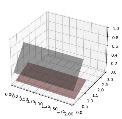
Done with procedural code following the references, for an unique timestamp.#
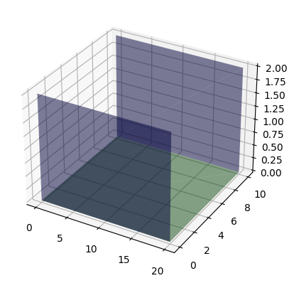
Done with Object-Oriented code, for an unique timestamp; plots the first example of the paper.#
The current code I have for the last plot looks like:
# %%
# Plot example problem
fig = plt.figure()
ax = fig.add_subplot(111, projection="3d")
# Params: center point, surface_azimuth, surface_tilt, axis_tilt, width, length
field = RectangularSurface([20 / 2, 10 / 2, 0], 0, 0, 0, 10, 20)
field.plot(ax=ax, color="forestgreen", alpha=0.5)
pv_row1 = RectangularSurface([20 / 2, 0, 2 / 2], 180, 90, 0, 2, 20)
pv_row1.plot(ax=ax, color="darkblue", alpha=0.5)
pv_row2 = RectangularSurface([20 / 2, 10, 2 / 2], 180, 90, 0, 2, 20)
pv_row2.plot(ax=ax, color="darkblue", alpha=0.5)

# %%
# Calculate the shadows
shades = field.get_shades_from(solar_zenith, solar_azimuth, pv_row1, pv_row2)
# TODO: shades union, intersection with the field surface and shade factor calculation
Regarding the diffuse component, I think I will leave it out for now. Maybe even for the whole GSoC period. I find it too tightly coupled to each spatial problem that coming up with a general approach seems unfeasible. And that the paper assumes an isotropic sky, which at this point seems like another source of error. Add the fact that it is a component that a good amount of time is not as relevant as the direct component. So I will focus on the direct component for now.
Next steps#
I will continue working on the direct beam shading factor for this month, while I also redact my final year dissertation and finish my internship (and move from the capital city). Yup, I’m going to have fun this month!